Page 4 - Open-Access-Nov-2020

TECHNICAL PAPER

Table 3: Probability of corrosion rate corresponding (iii) In the case of localized attack this will give an
to different ranges of resistivity underestimation of the pit depth as the area used is
the total area and not the area of the small corroding
RESISTIVITY PROBABILITY OF CORROSION
zone. In order to calculate the pit depth, an empirical
> 1000 – 2000 Ω.m The corrosion rates will be low. The concrete is dry relation can be used, which is used for most of the metal-
> 500 – 1000 Ω.m The concrete is moderately dry. Low corrosion rate aqueous systems. A pitting factor named α can be used,
whose value is around 10 times (in the case of concrete
> 100 – 500 Ω.m Concrete is wet. Corrosion rate will be moderate
structures):
< 100 Ω.m Wet concrete with high porosity. High corrosion rate
P pit = α × P corr = 10 P corr (8)
2.3 Polarization Resistance, R p As practical details it is important that:

Linear polarization technique is used to obtain the polarisation (i) The potentiostats to be used for R p measurements must be
resistance of the steel rebars, although the polarization curve able to calculate this ohmic drop, Re, or to compensate for
(current versus potential) does not have a linear relation. its influence during the recording of the R p measurement.
However, when the polarization is very small, the relation The method is usually applied through DC currents
between current and potential can be assumed to be linear although the ohmic drop can also be calculated from an
around the corrosion potential of the steel . It represents impedance result.
[9]
the “Resistance” to corrosion (polarization) and is given by
(ii) The registering of the current or potential has to be made
Equation (4):
after waiting a certain time (usually between 30 and 100 s)
(4) because it is necessary to wait until the full charge
0 dissipation of the capacitor – formed by the double layer
The corrosion rate is the inverse of this expression multiplied of the steel-concrete interface. A very short waiting period
by a factor (constant ‘B’) which can be taken as 26 mV as an leads to erroneous results perturbed by the capacitance
average. This is shown in Equation (5). contribution.

= 26
= (5) The typical ranges of corrosion rate in the laboratory and on-site
×
structures are given in Table 4.
The standard units of I corr are µA/cm or alternatively in µm/y.
2
The two units are related by the relation shown in Equation (6). The I corr value when integrated with the time gives the total
metal loss through Faraday’s law. Figure 7 gives the values of the
1 µA/cm = 11.6 µm/y (6)
2
evolution of the I corr for the same period as that shown in figure 4
The main aspects that must be taken into account are: and 5, and the corresponding integration at each time. This
mass loss can be expressed in loss of cross-section (diameter)
(i) The electrical resistance of the concrete must be (Figure 8) or corrosion penetration P corr (in mm or in µm). As
discounted as indicated in Equation (7) indicated in the Figure 7, the instantaneous corrosion rate is not
(7) a fixed value which remains constant, but it evolves with time
R p (measured) = R e + R p
due to the progression of the hydration with the reduction of
(ii) The R p value must be multiplied by the exposed area of the porosity and the increase in resistivity. It also is influenced
the metal as indicated in equation (5). The R p is expressed by the changes in temperature and humidity due to the climate
in KΩ.cm .
2
conditions in a parallel manner than the corrosion potential or
[12]
the resistivity.
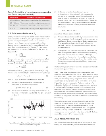
10000
The relation between the integrated corrosion rate and the
Resistivity ( Kohm.cm) 1000 correspondence of the total mass loss (gravimetric loss) is
metal loss can be expressed as well in Figure 9 where the
[9]
represented against the “electrochemical loss”. This type of
diagram is very important to calibrate the electrochemical
measurements and served in the initial times to identify the best

100 value of the constant ‘B’ in the equation (5).
0.00 1.00 2.00 3.00 4.00 5.00 6.00 7.00
2.3.1 Measurement on site
Time (y)
Figure 6: Evolution of the resistivity values in the carbonated specimen Due to its simplicity and accuracy, the LRP technique has been
and condition than that of figure 4. widely used in the laboratory for numerous metal/electrolyte

10 THE INDIAN CONCRETE JOURNAL | NOVEMBER 2020