Page 14 - ICJ Jan 2026

TECHNICAL PAPER

(26)

From Equations 24 and 25, A 1 (p)k p = a 1 (p), k p (air) = 0.0258, hence,
2
a 1 (p) = k p × A 1 (p) = 0.0258 × (30.99p – 0.46p + 2.29) i.e., a 1 (p) =
0.799p – 0.012p+0.059. For p = 0, a 1 (0) = 0.059 is nearly equal to
2
zero; and p = 1, a 1 (1) = 0.846, which is close to 1.
Thus, similarly as 1/λ 1d , 1/λ 1s can be written as 1/λ 1s = C 1 (p) k s +
D 1 (p) as 1/λ 1s varies linearly when the pores are saturated with
water, the conductivity of the pore is taken as water conductivity
i.e., 0.6051 W/m.K. For cell with water-filled enclosing pore,
(27)

(28)
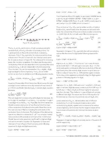
Figure 18: 1/λ 1d against k s
(29)
The λ 1d , λ 1s and λ 2s are functions of both porosity p and solid
conductivity k s , while λ 2d is function of porosity p alone. For Regression of slopes of 1/λ 1s against k s line with porosity in a
a given porosity as the solid conductivity k s increases λ 1d manner like that done for A 1 (p) yields following equation for
decreases. Plot of 1/λ 1d , against k s , for various porosities shows C 1 (p),
a linear trend. The plot is linear with the intercept nearly same
for all cases as shown in Figure 18. This is because for enclosing (30)
pores, the insulation properties of air dominate the equivalent
conductivity of the cell and depends more on porosity than solid B 1 (p) at p = 0, i.e., B 1 (0) = 1.15 and is not 1 as in case of simple
series model. B 1 (1) = 1.81 and again is not zero. As p ⟶ 1, the
conductivity. λ 2d , is almost independent of solid conductivity.
Thus, the term 1/λ 1d can be expressed as 1/λ 1d = A 1 (p)k s + B 1 (p); solid continues to contribute to effective conductivity of the cell,
significantly, thus this anomaly. B 1 (p) reduces to up to about p =
A 1 (p) and B 1 (p) functions of porosity. The λ 1d can be further 0.22 to a value of nearly 1.0, i.e., 1.09 and then again increases.
written as ratio from its definition and following equation results,
Performing similar regression as done for B 1 (p), for D 1 (p) against
p, leads to following equation for D 1 (p),
or (23)
(31)
Equation 23 resembles Ohm’s Series Law Model except for A 1 (p)
and B 1 (p) involve nonlinear terms of p instead of linear terms of D 1 (p) at p = 0, i.e., D 1 (0) = 0.84 and is not 1; and D 1 (1) = 0.24 and
p in Ohm’s Law Model. Introducing k p in constant A 1 (p), equation again is not zero. D 1 (p) decreases continuously from 0.84 at p = 0
becomes, to 0.24 at p = 1. Ratio of k p /k s is 23 times higher for saturated
case than dry case. Thus, behavior in case of D 1 (p) with porosity
(24) is different than B 1 (p). The nature and form of the equation for
the intercept as a function of p seems to vary with k p /k s ratio.
The term A 1 (p) shall increase with p while B 1 (p) shall decrease. At
p = 0, A 1 (p) = 0; and B 1 (p) = 1, so that k ec1 = k s ; and at p = 1, a 1 (p) = Linear variations of λ 2d i.e., dimensionless ratio of effective
1 and B 1 (p) = 0, so that k ec1 = k p . Physically, the Ohm’s Series Law conductivity of unit cell housing enclosed pores to solid
Model considers obstruction of heat flow by finite thick layer conductivity, k ec2 (dry)/k s , against solid conductivity for various
of low conductivity fluid placed in the path of heat flow, but in values of porosity, demonstrate that the negative slopes of the
this case volumes of fluid surrounding the solid obstruct the lines increase with porosity and intercept decreases as given
conduction from all directions. The thickness of the obstructing below,
1/3
layer in any direction is related to (1 – p) in a complex manner,
hence variation with porosity is nonlinear unlike in Ohm’s Law (32)
Model. Second order equations may fit well for A 1 (p) and B 1 (p) Regression of A 2 (p) and B 2 (p) with porosity results in Equations 33
and suit the model in Equation 23. Regression of slope and and 34 respectively,
intercept of lines in Figure 18 with porosity yields following
equations for A 1 (p) and B 1 (p) respectively, (33)

(25) (34)

THE INDIAN CONCRETE JOURNAL | JANUARY 2026 19