Page 15 - ICJ Jan 2026

TECHNICAL PAPER

The regression of λ 2s with solid conductivity leads to following water saturated effective conductivity k es , the k s and f can be
form of equation, obtained through a trial-and-error procedure as described
below and elaborated in the references [36,39] .
(34)
5.2 Application of the model to rock for
Further regression of C 2 (p), D 2 (p) and E 2 (p) result in following
equations, aggregate
Thermal conductivity of some rocks used as aggregates are then
(36)
obtained first. Measured thermal conductivity of some rocks are
(37) given in this section both in dry and saturated states, in Table 2.
Additionally, this table shows measured values of permeable
(38) porosity of these rocks. The methods used for measurement of
these properties are same as those used for concrete, that is the
In most of the regression equations coefficient of correlation
ranged from 0.95 to 0.99. More elaborate discussions on these hot wire line source method.
equations are available in references [36,39] . As an example, the dry and saturated conductivities of shale
rock are 3.22 and 4.69 W/m.K, respectively and the porosity is
Summarizing the model requires two inputs: k s the solid
conductivity and f, the fraction of enclosed pores, to estimate 4.84 %. Assume a value of 5.00 for k s . The calculated values of
thermal conductivity of porous building materials for a given A 1 (p), B 1 (p), A 2 (p), and B 2 (p) are given below.
porosity both in dry and water saturated states. For dry state A 1 (0.0484) = 30.99 × 0.0484 – 0.46 × 0.0484 + 2.29 = 2.34
2_
equations given below can be used,
2
B 1 (0.0484) = 1.17 × 0.0484 – 0.51 × 0.0484 + 1.15 = 1.13
2 –3
A 2 (0.0484) = (0.63 × 0.0484 + 3.3 × 0.0484 + 0.30) × 10 = 0.00046
2
B 2 (0.0484) = 0.33 × 0.0484 – 1.32 × 0.0484 + 1.01 = 0.9469
where, λ 1d and λ 2d are given as earlier,
With above values of A 1 (p), B 1 (p), A 2 (p) and B 2 (p), λ 1d , and λ 2d , are
; then calculated as,
where, A 1 (p), B 1 (p), A 2 (p) and B 2 (p) are as given before. A 1 (0.0484) k s + B 1 (0.0484) = 2.34 × 5 + 1.13 = 12.83;
Hence for known porosity all above terms A 1 (p), B 1 (p), A 2 (p) and λ 1d = 0.0779
B 2 (p) can be calculated and hence λ 1d and λ 2d can be estimated
Similarly, λ 2d = A 2 (0.0484) k s + B 2 (0.0484) = – 0.00046 × 5 + 0.9469
when k s is known, and if ‘f’ is known k ed can be estimated.
= 0.9446
Similarly, for saturated state the Equation given below can be
used to estimate corresponding saturated conductivity, Next step is calculation of λ 1s and λ 2s through C 1 (0.0484),
D 1 (0.0484), C 2 (0.0484), and D 2 (0.0484);

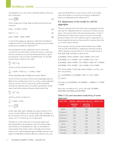
Table 2: Dry and saturated conductivity of some
where, λ 1s and λ 2s are given as,
aggregate
ROCK TYPE THERMAL CONDUCTIVITY (W/m.K) POROSITY (%)
OVEN DRY MOISTURE
STATE SATURATED
Basalt 4.03 5.00 0.40
where, C 1 (p), D 1 (p), C 2 (p), and D 2 (p) are as given before and for
known porosity all above terms C 1 (p), D 1 (p), C 2 (p), and D 2 (p) can Limestone 1 3.15 3.49 0.84
be calculated and hence λ 1s and λ 2s can be estimated when k s is Limestone 2 3.60 4.52 2.53
known, and if ‘f ’ is known k es can be estimated. Sandstone 1 4.45 7.86 10.56
Sandstone 2 3.16 4.55 7.01
The input k s to the model cannot be directly determined
from experiment as k s represents conductivity of pore free Shale 3.22 4.69 4.84
solid. Fraction of enclosed pores is also not amenable to Siltstone 1 3.45 5.29 5.10
direct experimental determination, although some indirect Siltstone 2 3.52 5.22 1.95
measure of ‘f ’ can be obtained experimentally. However, from
experimentally determined dry effective conductivity, k ed and Quartzite 8.58 8.64 0.30

20 THE INDIAN CONCRETE JOURNAL | JANUARY 2026